The following entry describes the concepts of molecular orbital theory for the structure and bonding in molecules. It is assumed that the Researcher has some prior knowledge of chemistry in order to fully appreciate the entire entry. Some further reading on the size of molecules, electron shells and orbitals and quantum mechanics may help.

Molecular orbital [MO] theory is a more developed and accurate theory for chemical bonding than valence bond [VB] theory and is used almost universally in theoretical and computational chemistry. Unlike VB theory, MO theory doesn't treat the electrons as belonging to specific bonds, but as being spread out over the whole molecule. The theory can be used to describe the chemical bonding in simple diatomic molecules (such as hydrogen and nitrogen molecules) and even in more complex organic and inorganic molecules. The theory can also be applied to transition metal complexes and can be extended to explain the bulk properties of solid materials such as semi-conductors.

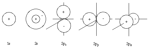
Wavefunctions¹ can be derived by solving the Schrodinger equation for an atom such as hydrogen and are called 'atomic orbitals'. If we solve the Schrodinger equation (using the Born-Oppenhiemer approximation) for the molecular ion H₂⁺ in which we have two protons and one electron, we get a set of wavefunctions called molecular orbitals. The probability of finding an electron at a given point in an atom is proportional to the square of the atomic orbital wavefunctions. In the same way, the probability of finding an electron at a given point within a molecule is proportional to the square of the wavefunctions of the molecular orbitals.

If we label the two nuclei in H₂⁺ 'A' and 'B', we can derive a ground state wavefunction for the electron in this molecular ion by a combination of the wavefunctions for this electron when it is totally on atom A and totally on atom B. This is written as:

ψ = ψ_A1s + ψ_B1s

What this equation tells us is that, if the electron is very close to nucleus 'A', ψ_B1s will be very small and the overall molecular orbital wavefunction will resemble that of ψ_A1s. Conversely, if the electron is close to nucleus 'B', the overall molecular wavefunction would resemble that for purely ψ_B1s. The formation of a molecular orbital in this way is called a linear combination of atomic orbitals [LCAO]. The MO formed above resembles an s-orbital when viewed along the axis running through both nuclei, and so it is called a σ-orbital, σ being the Greek letter for 's', 'sigma'. As this is the lowest energy molecular orbital it has the label 1σ. The electron configuration for H₂⁺ can be written in a similar way as for a hydrogen atom. For the H atom where the electron is in the 1s orbital, the electron configuration is 1s¹. In H₂⁺, the ground state electron configuration is written as 1σ¹.

The wavefunctions of atoms 'A' and 'B', as implied by the name, can be thought of as waves of electron density. When we form a molecular orbital, we get constructive interference between the waves of the two atoms. This leads to an enhancement in the amplitude of the electron density in the space between the two nuclei. The electrons can interact strongly with both nuclei so that there is a reduction in energy compared to that of the two separated atoms. The accumulation of electron density between atoms by the summation of their atomic wavefunctions is the key to the molecular orbital theory of chemical bonding.

Bonding and Antibonding Combinations of Atomic Orbitals

At first glance, there might seem to be little difference between valence bond theory and molecular orbital theory. When forming a bond in VB theory, we take two wavefunctions, one for each unpaired electron in the atomic orbitals on atoms 'A' and 'B', and form one VB wavefunction. In MO theory, however, if we have two atomic orbitals when forming a bond, we must form two molecular orbitals. The 1σ orbital in H₂⁺ is an example of what is called a bonding molecular orbital, where the atomic orbitals interfere constructively. In MO theory we can also form a second molecular orbital through the destructive interference between the atomic orbitals. This is called an antibonding molecular orbital where the wavefunctions for the atomic orbitals are subtracted from each other. In other words the signs for the amplitude of the two wavefunctions are opposite.

ψ^* = ψ_A1s - ψ_B1s

In contrast to the 1σ orbital, this antibonding orbital leads to a decrease in the amplitude of the wavefunction between the nuclei. In fact we get what is called a 'nodal plane' exactly half way between the nuclei, perpendicular to the bond. This is a region where the wavefunction amplitude falls to zero and so there the probability of finding any electron occupying the orbital is zero at this position. While the 1σ orbital is at lower energy than the two individual H1s orbitals, the antibonding combination lies at higher energy. Population of the antibonding orbital, therefore, leads to a weakening of the bond. Antibonding orbitals are often more antibonding than the bonding orbitals are bonding (ie, the energy gap upwards from the atomic orbitals to the antibonding orbital is greater than the drop down from the atomic orbitals to the bonding orbital). This is because the electrostatic repulsion between the nuclei pushes up the energy of both bonding and antibonding levels relative to the individual atomic orbitals. Hence the antibonding combination is more destabilised relative to the atomic orbitals than the bonding combination is stabilised.

Viewed along the bond, this molecular orbital resembles an s-orbital and is also a σ-orbital. It is labelled 2σ^*, the number 2 showing that it is the second lowest σ-orbital in energy with the asterisk denoting its antibonding nature.

Bonding in Diatomic Molecules

In describing electronic structure and bonding in molecules by molecular orbital theory, we follow a similar method for determining the electron configuration as we would for a single atom. We first create N molecular orbitals from linear combinations of N suitable valence atomic orbitals on the constituent atoms. We then fill these molecular orbitals with electrons from the bottom up to give the lowest energy configuration. As with the building up principle for atoms, we must follow the Pauli exclusion principle² and Hund's rules³.

First Row Diatomic Molecules - Hydrogen and Helium

We can construct energy level diagrams to help explain bonding. We draw the energy levels for the atomic orbitals for the participating atoms on the left and right hand sides with the energy levels for the resultant molecular orbitals in the centre. For the energy level diagram for hydrogen (figure 1) we have the H1s atomic orbitals for the individual atoms and in the centre the two molecular orbitals constructed from these. At lower energy, the bonding 1σ orbital and at higher energy the antibonding 2σ^* orbital. The two electrons are put into the 1σ orbital and are represented two arrows, one up and one down denoting their +½ and –½ spin states. This energy diagram helps us to visualise how the bond is formed through the reduction in energy by accommodating the electrons in lower lying molecular orbitals.

Figure 1: Molecular orbital energy diagram for H₂.

The energy level diagram for the hypothetical molecule He₂ is similar to that for H₂. Each helium atom contains 2 electrons in their 1s orbitals. When we put the four electrons into the molecular orbital in the energy diagram we get the ground state configuration 1σ²2σ^*2. The bond formed by the electrons in the 1σ orbital is cancelled out by the population of the 2σ^* orbital resulting in no overall stabilisation and hence no bond. In fact, since 2σ^* is more antibonding than 1σ is bonding, He₂ is at higher energy than the separated He atoms showing us why helium is a monatomic gas.

Second Row Diatomic Molecules

When looking at the diatomic molecules of the second row of the periodic table (Li to Ne), the valence orbitals with which we can form molecular orbitals are 2s and 2p. The 2s orbitals of each second row atom can overlap in a similar way to hydrogen to produce 1σ and 2σ^* orbitals. We also have three p-orbitals. By definition we label the internuclear axis of the molecule the z-axis and we see that the 2p_z orbital of one atom points straight at the 2p_z orbital of the other atom. Using these two orbitals, we can form a further two molecular orbitals, both with circular symmetry about the internuclear axis. These are therefore called 3σ (bonding and lower in energy than 2p_z) and 4σ^* (antibonding and higher in energy than 2p_z). The four σ orbitals, however, can't be strictly described as purely being derived from s or p_z-orbitals. Since the 2s or 2p_z-orbitals are both cylindrically symmetrical about the internuclear axis, the 2s orbitals of one atom can overlap with the 2p_z orbital of the other atom. We should therefore consider each of the four molecular orbitals, 1σ, 2σ^*, 3σ and 4σ^*, as being a combination of the 2s and 2p_z orbitals of both atoms. This is called s-p mixing and should be expressed mathematically as:

ψ = c₁ψ_2s(A) + c₂ψ_2s(B) + c₃ψ_2pz(A) + c₄ψ_2pz(B)

The coefficients, c, denote the contribution of each atomic orbital to the molecular orbital. The sizes of these coefficients for a given molecular orbital will depend on the energy separation of the s and p-orbitals of the individual atoms. For the molecular orbitals 1σ and 2σ^*, closer in energy to the 2s orbitals, the coefficients c₁ and c₂ will be large and c₃ and c₄ will be small. For the molecular orbitals 3σ and 4σ^*, close in energy to the 2p orbitals, the coefficients c₁ and c₂ will be small and c₃ and c₄ will be large. What this means is that 1σ and 2σ^* will be similar to the combinations of pure 2s and 3σ and 4σ^* will resemble the contributions from pure 2p_z. 2σ^* will therefore have some 2p_z character and 3σ some 2s character resulting in a slight shift in energy of these two orbitals.

We still have the 2p_x and 2p_y orbitals to consider. These are perpendicular to the internuclear axis and so can overlap side-on to give molecular orbitals. As with VB theory, these resemble p orbitals and so are called π-orbitals. For 2p_x we form bonding and antibonding combinations termed 1π and 2π^*. The same occurs with the 2p_y creating π-orbitals of exactly the same energy. So, each π energy level is composed of two molecular orbitals and have the same label and are said to be doubly degenerate.

The relative order of the σ and π orbitals can't be readily predicted due to varying strength of the s-p mixing. For the second row homonuclear diatomic molecules, it turns out that 3σ is higher in energy than 1π for N₂ and below (figure 2) and lower than 1π for O₂ and above (figure 3).

We have seen that the s and p_z orbitals form σ orbitals and the p_x and p_y orbitals form π orbitals. Why don't we form molecular orbitals by overlapping an s orbital with a p_x or p_y orbital? The s (and p_z) orbitals in diatomic molecules are cylindrically symmetrical along the internuclear axis, whereas the p_x and p_y each have a plane of symmetry. The wavefunction of the dumbbell-shaped p-orbitals have positive amplitude in one lobe on one side of the nucleus, and negative amplitude in the other lobe. If we try to overlap an s-orbital sideways with a p-orbital, the wavefunction of the s-orbital has equal overlap with both the positive and negative lobes of the p-orbital, resulting equal proportions of bonding and antibonding so there is zero net overlap.

Now we have defined the molecular orbitals, we can fill them with the valence electrons of the contributing atoms. For N₂ we have ten valence electrons. First, we put a pair of electrons in the 1σ orbital, then we fill the 2σ^* orbital (see figure 2). In N₂, the next energy level is 1π. This is doubly degenerate level has two molecular orbitals and so we can accommodate two electron pairs. The two remaining electrons are then put into the 3σ orbital giving the ground state configuration:

N₂ 1σ²2σ^*21π⁴3σ²

Figure 2: Molecular orbital energy diagram for N₂.

The strength of a bond is dependent on the bond order, b. This is defined as half the difference between the number bonding electrons, n, and antibonding electrons, n^*, and is basically the net number of bonding interactions.

b = ½(n - n^*)

For H₂ (1σ²), b = 1, but the two extra electrons for He₂ in 2σ^* give us a bond order of zero. For N₂, we have eight electrons in bonding orbitals and two electrons in an antibonding orbital. Hence we have a bond order of three agreeing with the triple bond predicted by VB theory, explaining its great strength (942kJ mol^-1) and hence inertness.

When moving from N₂ to O₂ (figure 3) we have two extra electrons to accommodate. The next highest level is 2π^* (note that the 3σ orbital is now lower in energy than the 1π orbital) and so we have the configuration:

O₂ 1σ²2σ^*23σ²1π⁴2π^*2

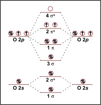
Figure 3: Molecular orbital energy diagram for O₂.

Since the 2π^* level is doubly degenerative, we put one electron in each π^* orbital with their spins parallel. This reduces the bond order to two, giving the expected double bond. The presence of two unpaired electrons makes it a di-radical, explaining its aggressive oxidative nature, and also predicts oxygen to be a paramagnetic substance which is indeed the case. This demonstrates the fundamental superiority of MO theory over VB theory, which predicts that all the electrons in O₂ should be paired.

For F₂, we have a further two electrons and these fill the 2π^* level, reducing the bond order to one and giving it a single bond, which explains the weak F-F bond (154 kJ mol^-1).

F₂ 1σ²2σ^*23σ²1π⁴2π^*4

Moving from F₂ to the molecule Ne₂, the two extra electrons fill the remaining molecular orbital available, 4σ^* to give the configuration:

Ne₂ 1σ²2σ^*23σ²1π⁴2π^*44σ^*2

This results in a bond order of zero, explaining the monatomic nature of neon. This can be extended to all the other elements of the Noble gas group to explain why they are all inert monatomic gases (although several highly unstable oxides and fluorides of krypton and xenon have been prepared in the past few decades).

Heteronuclear Diatomic Molecules

For diatomic molecules composed of atoms of different elements, we may have polar bonds. The bonding orbital in a polar molecule 'AB' is described by the wavefunction:

ψ = c_Aψ_A + c_Bψ_B

where the coefficients c_A and c_B are unequal. The proportion of each atomic orbitals contribution to the molecular orbital is given by the square of the coefficients. In a non-polar bond, c_B² = c_A² while in the purely ionic form A⁺B^-c_A² = 0 and c_B² = 1. In a polar molecule, the magnitude of the coefficients are somewhere between the two possibilities (see figure 4). In the molecule HF for example, the bonding occurs through a combination of the H1s and F2p_z orbitals. The participating orbital on fluorine is at lower energy to the hydrogen s-orbital and is therefore closer the energy of the 1σ orbital. The coefficient c_F is therefore much larger than the coefficient for the H atom and so the bonding orbital (and therefore the electrons in it) is mostly localised on the F atom. This is the cause of the bond's polarity. In the antibonding orbital 2σ^*, the coefficients are reversed so this orbital is mostly localised on the H atom.

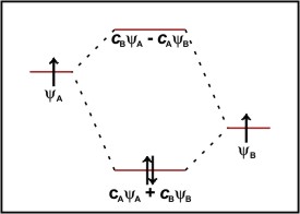
Figure 4: Molecular orbital diagram for a polar diatomic molecule such as HF.

Extension To More Complicated Systems

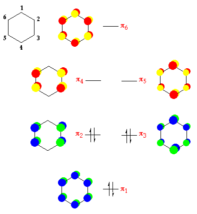
The principles of molecular orbital theory are easily extendable to more complicated organic and inorganic molecules. In benzene, we form a six-membered ring through σ bonded network of six carbon atoms leaving the six C2p_z to form six π-orbitals. We form a highly bonding orbital where all six orbitals interfere constructively and a highly antibonding orbital, where each p-orbital interferes destructively with the p-orbital on both neighbouring carbon atoms. Between these two levels are two doubly degenerate levels where we have two slightly bonding orbitals and two slightly antibonding orbitals⁴. The 6 π electrons fill the highly bonding and the two slightly bonding molecular orbitals, all of which are at lower energy than the p-orbitals of the separated atoms. This explains the stability of benzene and its relative inertness.

In transition metal chemistry we also have d-orbitals to consider. Four of the five d-orbitals have four lobes at right angles to each other where the opposing lobes have the same amplitude in the wavefunction and adjacent lobes have opposite amplitudes. (The other d-orbital resembles a p-orbital but with a ring around the middle. The two opposing lobes have the same amplitude whilst the ring about the centre has opposite amplitude). This presents the possibility of a third bonding interaction in addition to σ and π. If we overlap two d-orbitals of two transition metal atoms face-to-face, we can form molecular δ-orbitals. For example, in the ion [Re₂Cl₈]^2- (and also in its organometallic analogue [Re₂(CH₃)₈]^2-) each Re atom is bonded to four Cl atoms. The d orbitals of the Re atoms give rise a to σ combination, two degenerate π combinations and a δ combination resulting in a Re-Re quadruple bond.

MO theory can even be extended to study the bulk properties of solid materials such as metals, semiconductors and conducting polymers. We have seen that if we have N atomic orbitals, we form N molecular orbitals. If N is two then we form bonding and antibonding orbitals; if N is three then we form bonding, non-bonding and antibonding orbitals. In a solid material, we have so many molecular orbitals, each of which extends over the whole material, that the individual levels can be considered to form a continuous band. The population differences and energy gap between different bands in a material define the conducting or insulating properties of materials.

Conclusions

Molecular orbital theory provides a quantitative model for the chemical bonding in virtually all types of compound from simple diatomic molecules to more complex organic and inorganic compounds to large metal clusters. It allows the theoretical chemist to computationally model molecules and calculate their physical and spectroscopic properties and allows the modelling of the bulk properties of materials such as metals and semiconductors.

References

• Atkins, PW, Physical Chemistry, OUP

• Molecular Orbital Theory - www.chem.ufl.edu

• Molecular Orbital Theory - www.ch.ic.ac.uk